Convergence - Infinite Series Can Return a Finite Value
See Carnegie-Mellon's 'Numberous Proofs to the Basel Problem' for Mathematical History and Analytical Solutions
Demonstrated here: the power of calculus in resolving paradoxes created by infinity, and in obtaining analytical solutions to problems that are difficult to approach with numerical analysis alone. The following mathematical concept is convergence, and it applies to continuous functions as well as discrete sums.
Consider the following sequence:
$$\bbox[8px,border:1px solid black] { S_1 = \frac{1}{n^2}\,\ \,\text{where} \,\,n \in \Bbb{N}} \tag{Eq. 1}\label{s1}$$
Expanding this sequence starting at $n=1$ returns a simple list of fractions:
$$\bbox[8px,border:1px solid black] { S_1=\frac{1}{n^2} = 1,\,\frac{1}{4},\,\frac{1}{9},\,\frac{1}{16},\,\frac{1}{25},\,\frac{1}{36},\,...} \tag{Eq. 1.2}\label{1.1}$$
Now let us sum these set elements over the entirety of index n:
$$\bbox[8px,border:1px solid black] { \sum_{n=1}^\infty \frac{1}{n^2} = 1 + \frac{1}{4} + \frac{1}{16} + \frac{1}{25} + \frac{1}{36} + \dots} \tag{Eq. 2}\label{2}$$
On the surface, it looks like the series might sum to infinity regardless of how small these additions become; there are infinitely-many positive additions being made, after all. If adding-together an infinite sequence of numbers can return a finite sum, then what will that number be and how do we even attempt a solution?
- Moreover, these terms belong to the rational number set $\Bbb{Q}$. In finite math, we can't sum-together numbers from $\Bbb{Q}$ to obtain a number that is exclusively in $\Bbb{R}$. This is true for all natural numbers $\Bbb{N}$ and integers $\Bbb{Z}$ as well.

Calculus allows us to drop the discrete notation in favor of a continuous function which is analogous to our discrete series:
$$\bbox[8px,border:1px solid black]{ f(x)=\int_{1}^{x}\frac{1}{x^2} \ dx} \tag{Eq. 3}\label{3}$$
Below is a plot of $1/x^2$ with its underside shaded to represent the integral $\int{dx/x^2}$. This is our "area-under-the-function" interpration of integration. This graphical interpretation is often effective, but it doesnt provide any insight to our main question: does (Eq. 2) diverge towards infinity, or does it converge to some finite value?
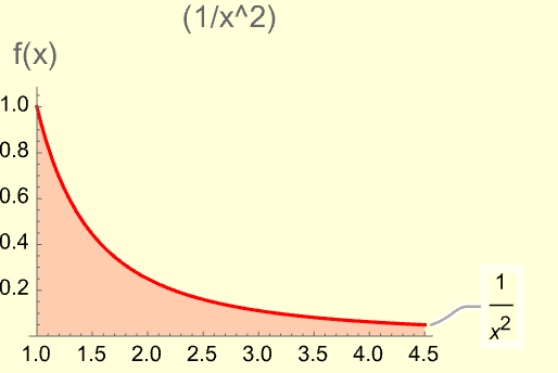
We need to integrate $f(x)$ over our domain $[1,\infty)$ and see what analytical solutions - if any - emerge.
Since $\infty$ is not itself a value of this expression, we could rewrite our improper integral
using limits and a dummy variable $t$, and evaluate:
$$\bbox[8px,border:1px solid black]{ \lim_{t \rightarrow \infty} \int_{1}^{t}\frac{1}{x^2}\ dx = \lim_{t \rightarrow \infty} \left[1 - \frac{1}{t}\right] = 1 - \cancelto{0}{\lim_{t \rightarrow \infty} \left[\frac{1}{t}\right]} = \bbox[#FF1,8px,border:0px solid red]{1}\ } \tag{Eq. 4} $$
Eq. 4 - If $t \rightarrow \infty$, then our quotient approaches zero and the integral is equal to 1.
Over the domain $[1,\infty)$, $f(x)$ encloses an area of exactly $1$. Until we evaluated the integral, there was no indication whether this would be our result. Obtaining an analytical solution to this problem using entry-level calculus is a strong indicator of the subject's importance and accessibility.
How Could We Demonstrate that this Solution is Not Trivial?
Ask: if $\int_{1}^{\infty} \left[\frac{1}{x^2}\right] dx$ converges to a real and finite value, then does $\int_{1}^{\infty} \left[\frac{1}{x}\right] dx$ also converge to a real, finite value? Consider these similarities:
- Both are rational expressions.
- Both are monotonically decreasing over $x \in [1,\infty)$
- $\lim_{x \rightarrow \infty} = 0$ and $\lim_{x \rightarrow 0} = \infty$ are true for both expressions
- Graphically, their shapes are very similar:
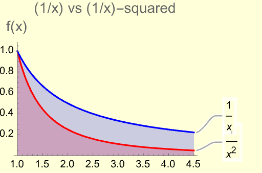
Reflecting on this page over the years, I still struggle to come up with new, "obvious" differences between these functions! Let us evaluate our continuous sum - $f(x)=\left[\frac{1}{x}\right]$:
$$\bbox[8px,border:1px solid black] { \lim_{t \rightarrow \infty} \int_{1}^{t} \left[\frac{1}{x}\right]\ dx = \lim_{t \rightarrow \infty} \ln[t]-\ln[1] = \infty - 0 = \bbox[#FF1,8px,border:0px solid red]{\infty} } \tag{Eq. 5}$$
Despite the lack of describable differences between tonicity, shape, and behavior at their boundaries , $f_1(x)$ converges over $[1,\infty)$ whereas $f_2(x)$ does not.
Evaluating Infinite Series Using Fourier Analysis
Integrating some function over $[1, \infty)$ is more conceptually abstract than summing a list of simple fractions.
Without proper context and exploration, it should be difficult to convince ourselves that (Eq. 4) really is related to the solution of the Basel Problem,
and just as difficult to accept that the solution to (Eq. 1) is some finite value rather than $\infty$.
Therefore, let us return to our discrete sum (Eq. 2) and attempt a solution using Fourier analysis.
We can relate our continous function, $f(x)$, to our discrete infinite series $S_1(n)$.
- Generally, Fourier analysis allows us to rewrite any continuous [Needs Citation] function - with arbitrary precision - as an infinite summation of sines, cosines and coefficients. Convenient for functions that are discontinuous (e.g., environmental vibrations).
- For a function $g(x)$ to have an associated Fourier Series, it must meet the Strong Dirichlet Conditions. Real (physical) signals will always satisfy these conditions! [Citation Required.]
$$\bbox[8px,border:1px solid black] { g(x) = \frac{a_0}{2} + \sum_{n=1}^{\infty} (a_n \cos(nx)+b_n sin(nx)) } \tag{Eq. 6}$$
The coefficients $a_0$, $a_n$ and $b_n$ are related to $g(x)$ via integration:
$$\bbox[8px,border:1px solid black] { a_0 = \frac{1}{2L} \int_{-L}^{L} g(x) dx } \bbox[8px,border:1px solid black] { a_n = \frac{1}{L} \int_{-L}^{L} g(x) cos\left[n \frac{x}{L}\right]dx } \bbox[8px,border:1px solid black] { b_n = \frac{1}{L} \int_{-L}^{L} g(x) sin\left[n \frac{x}{L}\right]dx } \tag{Eq.s 7-9}$$
Evaluating these three integrals yields one independent coefficient $(a_0)$ and two coefficients $(a_n, b_n)$ which vary with Fourier index $n$. The size of $n$ determines the precision of our series approximation of $g(x)$. Fourier analysis adapts the concept of convergence to fit approximation, computation and analytical purposes.
First introduced to me in Electrodyamics I: Parseval's theorem - valid only for square-integrable $g(x)$ - relates our function to the fourier coefficients as such:$$\bbox[8px,border:1px solid black] { \frac{1}{L} \int_{-L}^{L} \left[g^2(x)\right] dx = \frac{a^2_0}{2} + \sum_{n=1}^{\infty} \left[a^2_n+b^2_n\right] } \tag{Thrm. 1}$$
Given clever choices for $g(x)$, Parseval's theorem simplifies our mathematical approach to determining the value for a converging series.
- An advantage of (Thrm. 1) over (Eq. 6): our Fourier coefficients - $a_n$ and $b_n$ - now dominate their terms in the fourier series of $g(x)$. Integration terms simplify--therefore, our analysis and computational demands do as well.
Let's choose a function and analyze it with Parseval's Theorem to see if we can extrapolate information regarding why - and at what value - $S_1$ will converge.
- Let $g(x)$ = x
- Periodicity: $L= \pi$
$$\bbox[8px,border:1px solid black] { \frac{1}{\pi} \int_{- \pi}^{\pi} x^2\ dx = \frac{a^2_0}{2} + \sum_{n=1}^{\infty} \left[a^2_n+b^2_n\right] } \tag{Eq. 10}$$
Determine Coefficients $a_0$, $a_n$, and $b_n$ for $g(x)=x$
$$ \begin{align*} a_0 &= \frac{1}{\pi} \int_{- \pi}^{\pi} x\ dx\\ &= \frac{1}{\pi} \left[ \frac{x^2}{2} \right]\Bigg|_{-\pi}^{+\pi}\\ &= \frac{1}{\pi} \left[ \frac{\pi^2}{2} - \frac{(- \pi)^2}{2}\right]\\ & \bbox[8px,border:0px solid black] {= \bbox[#FF1,8px,border:0px solid red]{0} } \end{align*} $$
$$ \begin{align*} a_n &= \frac{1}{\pi} \int_{- \pi}^{\pi} x \cos{\left(n x\right)}\ dx\\ &= \frac {1}{\pi} \left[ \frac{\cos{\left(n x\right)}}{n^2} + \require{cancel} \cancelto{0}{\frac{ x \sin{\left(n x\right)}}{n}} \right] \Bigg|_{-\pi}^{+\pi}\\ &= \frac{1}{ \pi} \left[ \frac{ \cos{( - \pi n) } - \cos{( + \pi n) }}{n^2} \right]\\ &= \bbox[8px,border:0px solid black] { \bbox[#FF1,8px,border:0px solid red]{0} } for\ all\ n \end{align*}$$
$$ \begin{align*}
b_n &= \frac{1}{\pi} \int_{- \pi}^{ \pi} x \sin{\left(n x\right)}\ dx\\
&= \frac {1}{\pi}
\left[ \frac{ - \pi \cos{\left(n x\right)}}{n}
+ 0 \right]
\Bigg|_{-\pi}^{+\pi}\\
&= \bbox[8px,border:0px solid black] { \bbox[#FF1,8px,border:0px solid red]{ - \frac{2}{n} \cos{\left(n \pi\right)}} }
\end{align*} $$
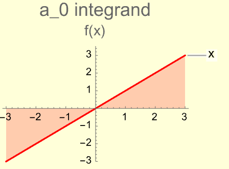
Notice that $a_0$ = $a_n$ = 0 in this case because of the integrand's symmetry about the origin. Here, $g(x)=x$ is an odd function ($g(-x)=-g(x)$). Symmetry is often leveraged to simplify, or make trivial many integral computations.
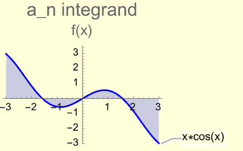
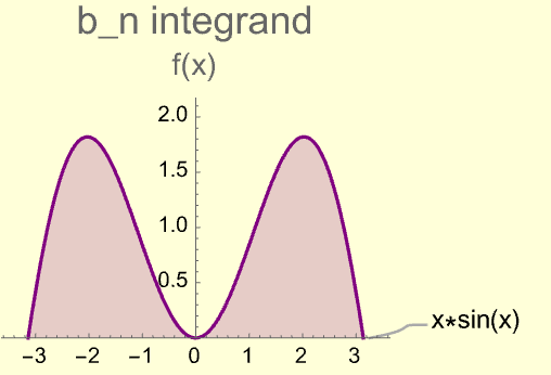
Graphically, it is clear to see that $a_0 = a_n = 0$ while $b_n \not= 0:$.
How a Solution to the Basel Problem Emerges from Parseval's Theorem
Substituting $a_0$, $a_n$, $b_n$ and $g(x)=x$ into (Thrm. 1), we are equating a simple integral to our infinite series:
$$\bbox[8px,border:1px solid black] { \frac{1}{\pi} \int_{- \pi}^{\pi} x^2\ dx = 4 \sum_{n=1}^{\infty} \left[ \frac{ \cos^2{(n \pi)}}{n^2} \right] = \frac{2 \pi^2}{3} } \tag{Eq. 11}$$
Encoded in (Eq. 11): the infinite sum of terms in $\left[cos{(n \pi)}/ n\right]^2$ for $n = (1, 2, 3, 4... \infty)$ is equal to a finite number - exactly $ \frac{ \pi^2}{6}$! Parseval's Theorem allowed us to simply integrate $ \int x^2dx$ to reach our conclusion.
- Congratulations! We have proven that certain infinite series will converge to a finite number.
- Possible because $\int x^2 dx$ is easily obtainable in comparison to $ \sum_{n=1}^{ \infty} \frac{cos^2(n)}{n^2}$
- We can take this a step further to actually solve the Basel Problem (Eq. 2) by analyzing $cos(n \pi)$ a little closer. Consider a table of cosine outputs for different $n$:
Cosine has a period of only $2 \pi$, so this table contains our only two unique outputs of $ \cos(n \pi)$:
Incredibly, the result is an irrational number! It is not trivial at this point that $\pi$ should appear. Why?
- Every term in our series belongs to the rational number set $\Bbb{Q}$, but our sum converges outside of that set to an irrational number in $\Bbb{R}$!
Leonhard Euler, (1707-1783)
Note that convergence was a known property of infinite series prior to Euler.
His discovery (in this context) is solving the Basel Problem.