Damped Harmonic Oscillator
Constructing and Justifying our Differential Equation
Hooke's law describes a restorative force: $F=-kx$. What makes this force restorative?
- As our system is displaced from equillibrium ($x_0=0$), a force directed towards $x_0$ grows proportionally to k. The force acts to restore the system to its equillibrium configuration.
Each contribution to the net force $\vect{F}$ may be written:
- $F_{spring}(x)= -kx$: A restorative force that depends explicitly on position.
Proportional to our spring constant $k$. - $F_{damp}(v)= -\beta \dot{x}$: A frictional force which grows in opposition to velocity.
Proportional to some damping factor $\beta$.
Newton's Equation for our spring system follows:
$$ F_{total} - F_{spring} - F_{damp} = 0$$ $$m \ddot{x} + \beta \dot{x} + kx = 0 $$ $$\blbox{m \frac{d^2 x}{dt^2} + \beta \frac{dx}{dt} + kx = 0} \tag{Eq. 1} $$Eq. 1 - Linear, second-order, ordinary differential equation. Force assocaited with a mass on a spring, with friction accounted for in our second term.
Undoubtably, constructing (Eq. 1) was far easier than jumping straight to its solution, x(t). In solving (Eq. 1), we will demonstrate that x(t) is not trivial, and would not have been easily-obtainable with algebra or empirical methods alone.
- Constructing differential equations is where much of our physics efforts get concentrated. A computer (or mathematician) can often do the brute work of actually solving the equations that we create to model our system. Refer to the Spherical Bessel Functions.
- However, physical intuition is often required to simplify equations and make them solvable.
Complex-Valued Solution to the Differential Equation for Real Spring Motion
For completeness, it is necessary to consider x(t) to be complex-valued when solving our differential equation. However, our physical (observable) system is described only by its real part (not its imaginary). We will write Re[x(t)] after working out our complex solution.
First observation: (Eq. 1) is actually homogonous in addition to being linear and ordinary. Given these properties, our complete (most general) solution must satisfy the following:
- Second-order, Linear diff. eq.: full solution must be a superposition of two linearly-independent solutions: $x_{full}(t)=C_1x_1(t)+C_2x_2(t)$. We will produce two complex-valued constants ($C_1,C_2$). Initial conditions and constraints on our system will lead to determinations of these constants. $C_1$ and $C_2$ determine the weight of each linearly-independent solution to our (Eq. 1).
- Ordinary diff. eq..: usually far easier to appraoch and solve than partial differential equations. The solution set will be finite as opposed to infinite (in the case of PDEs).
Examine the most genearlized oscillatory function we can come up with. In $\Bbb{R}^2$, we expect to find that it has two solutions, as it is a second-order ordinary differential equation (ODE): $$x_n(t)=C_n e^{i \omega_n t} \tag {Eq. 2.1}$$
Eq. 2.1 - $C_n$ are complex-valued constants, and may have imaginary parts!
Our most generalized solution, then, is some linear combination of these two solutions: $$\blbox{x(t)=C_1 e^{i \omega_1 t} + C_2 e^{i \omega_2 t}} \tag{Eq. 2.2} $$Reduction to an Eigenvalue Problem
Substitute this full solution into our equation of motion to start determining our solution parameters ($C_n, \omega_n$):
$$ \frac{d^2}{dt^2} [C_n e^{i \omega_n t}] + \left(\frac{\beta}{m}\right) \frac{d}{dt} [C_n e^{i \omega_n t}] + \left(\frac{k}{m}\right) [C_n e^{i \omega_n t} ]= 0 $$ Perform our time-derivatives in terms one and two: $$ i^2 \omega_n^2 [C_n e^{i \omega_n t}] + \left(\frac{\beta}{m}\right) i \omega_n[C_n e^{i \omega_n t}] + \left(\frac{k}{m}\right) [C_n e^{i \omega_n t} ]= 0 $$ Pull out common factors to reveal a quadratic equation, and our eigenvalue problem. Recall $i^2=-1$: $$\blbox{C_n e^{i \omega_n t} \left( - \omega_n^2 + i\frac{\beta}{m}\omega_n + \frac{k}{m} \right) = 0} \tag {Eq. 3.1} $$We need to eliminate this exponential term in order to solve the auxillary (or secular) equation (3.2).
- Algebraically, this is no problem: divide both sides by $C_n e^{i \omega_n t}$ to obtain (Eq. 3.2).
- Less hand-waivy: the quantity $e^{i \omega_n t}$ can never equal zero, so the only zeros (roots) in (Eq. 3.1) must follow from particular choices of $\omega_n$ (our eigenfrequencies):
Eq. 3.2 - Polynomial which is degree-two in $\omega_n$.
The upcoming math may be simplified by defining the following, algebraic substitutions: $$\begin{align} \beta /m \rightarrow 2\gamma \\ k/m \rightarrow \kappa^2 \end{align}$$Solve the auxillary equation to obtain two complex-valued eigenvalues:
$$ - \omega_n^2 + 2i\gamma \omega_n + \kappa^2 = 0 $$ $$\blbox{\omega_{1,2} = i\gamma \pm \sqrt{\kappa^2 - \gamma^2}} \tag {Eq. 3.3}$$ Therefore, our general solution for damped spring motion is given by substituting (Eq. 3.3) in (Eq. 2.2): $$ x(t)= C_1 e^{i^2 \gamma t} e^{+i \left(\sqrt{\kappa^2 - \gamma^2}\right)t} + C_2 e^{i^2 \gamma t} e^{-i \left(\sqrt{\kappa^2 - \gamma^2}\right)t} $$ $$ \blbox{x(t)= e^{-\gamma t} \left(C_1 e^{+i \left(\sqrt{\kappa^2 - \gamma^2}\right)t} + C_2 e^{-i \left(\sqrt{\kappa^2 - \gamma^2}\right)t} \right) } \tag{Eq. 4}$$ We already see an interesting quality of our solution to damped motion: our particle is oscillating with some new (relative to undamped motion) frequency that is related by its natural frequency ($\kappa$) and the systen damping (encoded in $\beta$).Interestingly, x(t) is a product of two distinctly-shaped functions: a factor that decays purely-exponentially in time, and a purely-oscillatory factor:
- $e^{-\gamma t}$ - Factor corresponding to pure exponential decay over time. A damping term, independnet of $\kappa$.
- $\left(C_1e^{...} +C_2e^{...} \right)$ - Factor corresponding to undamped oscillation of the system in time. Determined by both $\gamma$ and $\kappa$.
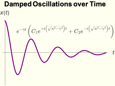
Figure 1 - Plot of (Eq. 4) for arbitrary parameters ($\gamma \lt \kappa$). Predicts oscillating motion that decays in amplitude over time. Matches our expectation of how a damped harmonic oscillator will behave. Changes shape if $\gamma \ge \kappa$ (critical/overdamping).
The Real-Valued Part of x(t)
Our complex-valued solution is the most complete description for damped oscillations in 1-D. However, the imaginary part ( Im[x(t)] ) does not contribute to any observable behavior, so we may disregard it and pursue a trigonometric form for (Eq. 4). To drop the imaginary part and clean notation, make the following substitutions:
$$ x(t) \rightarrow \text{Re}[x(t)] $$ $$ C_n \rightarrow A_n+iB_n $$ $$ \sqrt{\kappa^2 - \gamma^2} \rightarrow \Omega$$Note that $A_n, B_n$ are real-valued coefficients. The damped frequency, $\Omega$, varies between the natural frequency and 0 for positive damping (i.e., $\gamma>0$).
Damping results in energy loss, meaning the damped frequency ($\Omega$) is always
less than the natural (undamped) frequency ($\kappa$).
This mathemtical result makes intuitive sense (a luxury of solving classical systems).
Given these substitutions, the real-valued part of (Eq. 4) may be expressed in a very manageable form:
I have carefully grouped terms in (Eq. 5) such that it is clear which of our trigonometric terms are purely real versus purely imaginary -- our real solution for x(t) is clearly visible:
$$x(t) = e^{-\gamma t} \left[ (A_1 + A_2) \cos{\Omega t} + (B_1 - B_2) \sin{\Omega t} \right] $$ Compressing our solution constants yet again, we obtain an elegant solution to damped harmonic motion: $$\blbox{x(t) = e^{-\gamma t} \left[ A\cos{\Omega t} + B{\sin{\Omega t}} \right]} \tag {Eq. 6} $$Eq. 6 - The real-valued solution to Newton's equation for damped, harmonic motion (Eq. 1). The damped oscillation-frequency ($\Omega$) may be imaginary, necessitating the use of complex analysis (or Eq. 4) to evaluate behavior when $\gamma > \kappa$.
- Coefficients A and B are the only quantities that remain unknown. It makes sense that we still have some undetermined information in our solution, as we have yet to describe an actual system configuration. Therefore, A and B adjust the solution to match different initial conditions or constraints which define a given system.
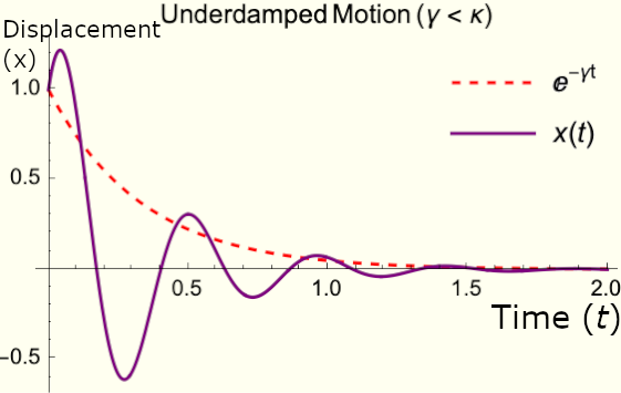
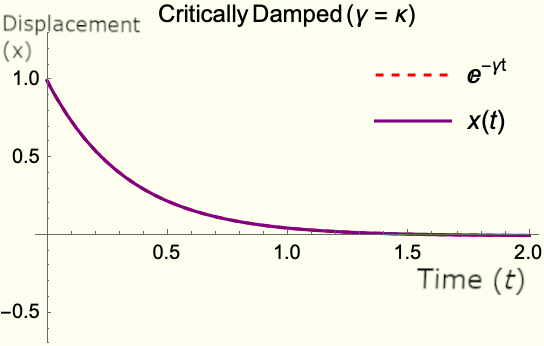
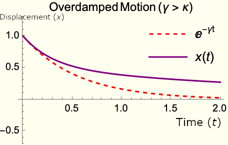
Figure 2 - Plots of x(t) for different damping strengths. The complex nature of x(t) encodes our lack of real roots in the overdamped case, and we lose our oscillatory behavior, slowing the system before equillibrium is reached (hence no real roots).
Our eigenfrequency $\Omega$ is influenced by the damping strength, implying that the mechanism for energy loss causes decay in amplitude in addition to down-shifting the oscillation periodicity from its undamped value (when $\gamma=0$). Indeed, the overdamped case is an exaggerated form of why amplitude decay must be occompanied by a down-shift in oscillation frequency.
Brief Verification of our Solution
Prior to a discussion, we should demonstrate explicitly that x(t) really does solve (Eq. 1). Use the complex-valued form (Eq. 4) over the real part (Eq. 6) in order to keep terms compact and avoid errors.
$$ \ddf{x}{t} + 2\gamma \frac{dx}{dt}+\kappa^2 x = 0$$ $$ \frac{d^2}{dt^2} \left[ e^{-\gamma t} \left( C_1 e^{i \Omega t} + C_2 e^{-i \Omega t} \right) \right] + 2\gamma \frac{d}{dt} \left[ e^{-\gamma t} \left( C_1 e^{i \Omega t} + C_2 e^{-i \Omega t} \right) \right] + \kappa^2 \left[ e^{-\gamma t} \left( C_1 e^{i \Omega t} + C_2 e^{-i \Omega t} \right) \right] \stackrel{?}{=} 0 $$ $$ -\left( \Omega^2 -\kappa^2 + \gamma^2) e^{-\gamma t} (C_1 e^{i \Omega t} + C_2 e^{-i \Omega t} \right) \stackrel{?}{=} 0 $$ $$ \cancelto{0}{([ \kappa^2 - \gamma^2 ] -\kappa^2 + \gamma^2)} e^{-\gamma t} \left( C_1 e^{i \Omega t} + C_2 e^{-i \Omega t} \right) \stackrel{\unicode{10004}}{=} 0 $$ Therefore, x(t) is a solution to (Eq. 1) for any choice for $\beta, m, k$, and t.Understanding Initial Conditions -- A, B
For a brief moment, consider how certain configurations of A and B influence x(t) at initial time $t=t_0$:
- If A = 0: $x(0) \rightarrow B\sin{0}$. The system starts at equillibrium ($\sin{0}=0$).
- If B = 0: $x(0) \rightarrow A\cos{0}$ = A. The system begins at its maximum value for displacement.
- A,B $\not =$ 0: $x(0) \rightarrow A$, while $\dot{x}(0) \rightarrow -B\Omega $. System begins with some velocity value.
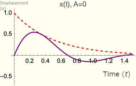
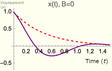
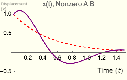
Figure 3 - Plots of motion for different values of A,B, illustrating that these parameters vary according to initial system configuration.