Vibrations of a Rectangular Membrane
Problem from Mathematics for Quantum Mechanics: An Introductory Survey of Operators, Eigenvalues, and Linear Vector Spaces (1962)
Problem 2-1: Show how eigenfrequencies of oscillation occur for the small oscillations of a uniform, flexible, rectangular membrane with sides of length a and b. Find the most general solution for the displacement, and show that the eigenfrequencies can be written $$ \omega_{mn} =\pi v \sqrt{\frac{m^2}{a^2}+\frac{n^2}{b^2}} $$ where m and n are positive integers (pp. 6).
Characterizing the System
This is an exercise in solving the wave equation for two spatial dimensions (vibrating plane embedded in $\Bbb{R}^3$).
Eigenvalues arise
as a result of our spatial boundary conditions (and single-valuedness of displacement). Two indices of eigenvalues are needed to account for two, independent spatial dimensions.
The motion of our membrane (uniform mass density $\rho$, subject to uniform tension T) is described by a linear, homogeneous, second-order partial differential equation (2-D wave equation):
$$T \left( \ddp{u}{x} + \ddp{u}{y} \right) - \rho \ddp{u}{t} = 0 \tag{Eq. 1} $$Rewrite (Eq. 1) to include a velocity term (rather than tension and density) -- $v^2 = T / \rho$:
$$\ddp{u}{x} + \ddp{u}{y} - \frac{1}{v^2} \ddp{u}{t} = 0 \tag{Eq. 1.1} $$Eq. 1.1 - Dimensionally, we have $[T][u][x]^{-2}= [\rho][u][t]^{-2}$, or $MLT^{-2}LL^{-2}=ML^{-1}LT^{-2}$ (SI units of $kg / s^2$). Equation is balanced and provides physical interpretation to the velocity term $[v]=LT^{-1}$.
Identifying Our Separable Differential Equation
$$u\left(x,y,t\right)=X(x)Y(y)Z(t)$$ $$ X''YZ + XY''Z - \frac{1}{v^2}XYZ'' = 0 $$ $$\blbox{ \frac{X''}{X} + \frac{Y''}{Y} - \frac{1}{v^2}\frac{Z''}{Z} = 0 }\tag{ Eq. 2}$$ Varying x, y, t independently from one-another must keep (Eq. 2) satisfied.Therefore, each term in (Eq. 2) must be constant, otherwise our statement would be impossible for all variable configurations. This is our standard argument for invoking separation of variables in PDE. $$ \left(k^2_x + k^2_y\right) - \frac{1}{v^2}\left(k^2_t \right)= 0 \tag{Eq. 2.1}$$ This leads to three linear, second-order ordinary differential equations for each system variable:
$$ \begin{cases} X'' + k^2_x\ X(x) = 0 \\ Y'' + k^2_y\ Y(y) = 0 \\ Z'' + v^2 k^2_t\ Z(t) = 0 \end{cases}$$
Solving for X and Y (Spatial Components)
Real-valuedness is a requirement of displacement, so I am skipping straight to trigonometric expressions for u. $$\begin{align} X(x) &= A_x \sin{(k_x x)} + B_x \cos{(k_x x)}\\ Y(y) &= A_y \sin{(k_y y)} + B_y \cos{(k_y y)} \end{align} \tag{Soln.1}$$Soln. 1 - Six unknowns. Determined by our boundary conditions (and the single-valuedness of u).
Our membrane is pinned at its parameter: $u(0,0,t)=u(a,b,0)=0$.
$$\begin{align} X(0) &= 0= A_x \cancel{\sin{0}} + B_x \cancelto{1}{\cos{0}} \\ Y(0) &= 0 = A_y \cancel{\sin{0}} + B_y \cancelto{1}{\cos{0}} \end{align}$$ $$\blbox{ \begin{align} B_x = 0 \\ B_y = 0 \end{align}} \tag{Soln. 1.2}$$Soln. 1.2 - No cosine contribution, since we need exactly 0 displacement along the pinned edge. Information about A is not provided by this boundary condition.
The wavenumbers $k$ follow from this constraint:
$$\begin{align} X(a) &= 0 = A_x\sin{(k_xa)} \\ Y(a)&= 0 = A_y\sin{(k_yb)} \end{align} $$This condition forces quantized values of $k$, since (Eq. 3) is satisfied by any integer m in sin(m$\pi$). In quantum mechanics, this result is why we obtain quantized energies when solving for matter (particle) waves.
$$k_{j}\ell = j\pi $$ $$\blbox{ \begin{align} k_x &= m\pi /a \\ k_y &= n\pi /b \\ \end{align} } \tag{Soln. 1.3}$$ Finally, $A_x$ and $A_y$ can be found by substituting (Soln. 1) into each of our ODEs and evaluating: $$-k^2A +k=0$$ $$ \blbox{ \begin{align} A_x &= a/ m\pi \\ A_y &= b/ n\pi \end{align} } \tag{Soln. 1.4} $$ Substituting $A_{nm}$ and $k_x, k_y$ into $u(x,y,t)$: $$\bblbox{u(x,y,t)= \sum_{n,m}^{\infty} u_{nm}=\frac{1}{\pi^2} \sum_{n=1}^{\infty} \sum_{m=1}^{\infty} \left( \frac{ab}{mn} \right) \sin{\left(\frac{m\pi\ x}{a}\right)} \sin{ \left( \frac{n\pi\ y}{b}\right) } Z(t)} \tag{Soln. 1.5}$$Soln. 1.5 - Quantized wavenumbers (eigenvalues) and coefficients $A_{x,y}$, forced by our spatial boundary conditions. Z(t) must have dimensions of inverse length in order for this to work.
To solve our system, we just need to know how u evolves in time. In verifying our spatial solution, we can plot the normal modes:
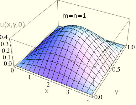
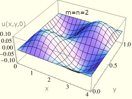
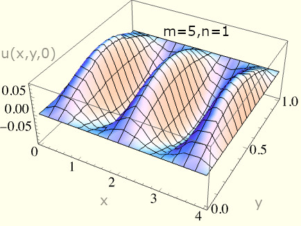
Fig. 1 - Plots showcasing some of the allowed membrane shapes as it vibrates with a particular eigenfrequency. Notice that the boundary condition holds true as we arbitarily vary m, n, a, b.
Solving for Z(t) (Time-Component)
$$Z'' + \left(v^2 k_t^2 \right)Z(t) = 0 $$ Dimensional analysis reveals that the quantity $vk_t$ is an angular frequency ($\omega_0$): $$[vk_t]^2 =L^2T^{-2}(L^{-2}) = 1/T^2 $$ $$Z(t)= C_1 \sin{(\omega t)} + C_2 \cos{(\omega t)} \tag {Soln. 2}$$The two initial conditions need to be invoked to obtain the two coefficients:
$$u(x,y,0)=f_0(x,y) \tag{I.C. 1}$$ $$\dot{u}(x,y,0)=g_0(x,y)\tag{I.C. 2}$$Keeping the coefficients $A_m,A_n$ in-tact, we can rewrite u(x,y,0) from (soln. 1.5) as double Fourier series:
$$ u(x,y,0) = f_0(x,y) = \sum_{n=1}^{\infty} \sum_{m=1}^{\infty} C_2 A_m A_n \sin{\left(\frac{m\pi\ x}{a}\right)} \sin{ \left( \frac{n\pi\ y}{b}\right) } \tag{Eq. 3.1.1}$$ $$ \dot{u}(x,y,0) = g_0(x,y) = \sum_{n=1}^{\infty} \sum_{m=1}^{\infty} \omega C_1 A_m A_n \sin{\left(\frac{m\pi\ x}{a}\right)} \sin{ \left( \frac{n\pi\ y}{b}\right) } \tag{Eq. 3.1.2}$$Eq. 3.1.2 - The factor of $\omega$ comes from operating on the first term in Z(t): $ \frac{d}{dt}\left[C_1 \sin{\omega t}\right] $.
Since the spatial boundary conditions brought on the discrete nature of $k_{x,y}$ (pp. 5), leading to the same behavior in $A_{mn}$, it should be safe to combine the coeffients $(A_mA_nC)$. In other words, I'm assuming that another index is not needed in order to account for the coefficients $C_1,C_2$ (unverified).
$$\begin{align} \left(C_2A_mA_n\right) &\rightarrow \alpha_{mn} \\ \left(C_1A_mA_n\right) &\rightarrow \beta_{mn} \end{align} \tag{Eq. 3.2}$$Eq. 3.2 - The convenience of rewriting the product of coefficients is why we chose not to expand (Soln. 1.4) when looking for time-dependent solutions, despite the valid finding that $A_xA_y=A_{mn}=\frac{ab}{mn\pi^2}$.
Obtaining $\omega_{mn}$ and a General Solution for u(x, y, t)
$$\bblbox{u(x,y,t)= \sum_{n=1}^{\infty} \sum_{m=1}^{\infty} A_{mn} \sin{\left(\frac{m\pi\ x}{a}\right)} \sin{ \left( \frac{n\pi\ y}{b}\right) } \left[ C_1 \sin{(\omega t)} + C_2 \cos{(\omega t)} \right] } \tag{Soln. 2}$$Soln. 2 - The most general solution to our PDE. This can be written in a more insightful form (revisited at the end of this page).
Substitution of (Soln. 2) into (Eq. 1) leads to the eigenfrequencies $\omega$, therefore demonstrating the quantized nature of the parameter. $$0 = \ddp{u_{mn}}{x} + \ddp{u_{mn}}{y} - \frac{1}{v^2} \ddp{u_{mn}}{t} \Bigg|_{t=0}$$* Evaluating at t=0 allows us to drop the time-depenendent trig terms. Harmonic frequency will not change with time, so this is a valid way to simplify the algebra involved in isolating $\omega_{mn}$. Verified in this problem's Mathematica notebook.
$$ \begin{align} 0 &= \alpha_{mn} \left( \frac{m^2}{a^2} \right) \sin{\left(\frac{m\pi\ x}{a}\right)} \sin{ \left( \frac{n\pi\ y}{b}\right) } \\ &+ \alpha_{mn} \left( \frac{n^2}{b^2} \right) \sin{\left(\frac{m\pi\ x}{a}\right)} \sin{ \left( \frac{n\pi\ y}{b}\right) } \\ &- \alpha_{mn} \left( \frac{\omega^2}{\pi^2 v^2} \right) \sin{\left(\frac{m\pi\ x}{a}\right)} \sin{ \left( \frac{n\pi\ y}{b}\right) } \end{align} $$ $$ 0 = \alpha_{mn} \sin{\left(\frac{m\pi\ x}{a}\right)} \sin{ \left( \frac{n\pi\ y}{b}\right)} \left[ \frac{m^2}{a^2} + \frac{n^2}{b^2} - \frac{\omega^2}{\pi^2 v^2} \right] \tag{Eq. 4} $$Eliminating the factor $\left[\alpha_{mn} \sin{\left(\frac{m\pi\ x}{a}\right)} \sin{ \left( \frac{n\pi\ y}{b}\right)}\right]$ reduces this to an eigenvalue problem for $\omega_{mn}$, which should be expected. $$ 0 = \frac{m^2}{a^2} + \frac{n^2}{b^2} - \frac{\omega^2}{\pi^2 v^2} \tag{Eq. 4.1}$$ $$ \bblbox{ \omega^2_{mn} = v^2 \pi^2 \left( \frac{m^2}{a^2} + \frac{n^2}{b^2} \right)} \tag{Solution} $$
- As expected, the 2-D wave behaves similar to the 1-D case. The system only oscillates harmonically at discrete frequencies.
- The elegance of the characteristic equation (Eq. 4.1) follows due to the wave equation's linearity and separability; demonstrably powerful properties of PDEs.
Extending Jackson's Problem (2-1): Fourier Coefficients
Revisiting (Eq. 3.1), we obtain clean, double-Fourier series to describe the initial spatial form of the wave: $$ u(x,y,0) = f_0(x,y) = \sum_{n=1}^{\infty} \sum_{m=1}^{\infty} \alpha_{mn} \sin{\left(\frac{m\pi\ x}{a}\right)} \sin{ \left( \frac{n\pi\ y}{b}\right) }$$ $$ \dot{u}(x,y,0) = g_0(x,y) = \sum_{n=1}^{\infty} \sum_{m=1}^{\infty} \omega_{mn} \beta_{mn} \sin{\left(\frac{m\pi\ x}{a}\right)} \sin{ \left( \frac{n\pi\ y}{b}\right) }$$The initial position and velocity of the wave ($f_0,g_0$) are given.
- Mathematically, we need to perform operations which isolate $\alpha_{mn}$ and $\beta_{mn}$. The eigenfrequencies ($\omega_{mn}$) are already known.
- Isolating the Fourier coefficients is typically achieved by invoking an orthogonality argument.