Dimensional Analysis and Limiting Conditions
Here's a powerful tool to demonstrate why theoretical physics is an effective approach when modeling real systems. There are advantages to working with dimensional quantities over unitless mathematical objects.
- In physics, we can verify our quantitative work by checking for balanced units in our expressions. This is invaluable in experimental physics, since your own computations via programming are dimensionless; the researcher must interpret instrumental results, and perform the dimensionally-correct calculations. Even raw data are stored as dimensionless number sets.
- We will explore extreme cases of system parameters - e.g., infinite mass, zero gravity - as a means of verifying that our mathematical results make physical sense.
- Deeper than that: we can find physical relationships in real systems using unit-balancing as our rationale for constraining variables.
Case I: The Pendulum
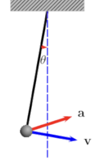
Using dimensional analysis and basic linear algebra, let us determine the exact form for a pendulum's cycle frequency. Physical observation will guide our mathematical logic, and vise versa.Consider: what real-world parameters determine a pendulum's frequnecy ($f$)? What system variables will $f$ vary with? Here are some reasonable predictions:
- Local gravitational acceleration ($g$)
- Length ($ \ell $) of the pendulum
- Mass ($m$) of the pendulum
- Initial angle $\theta_i$
Conveniently, all quantities except for $ \theta$ are dimensional. Whatever form $f( \ell,g,m, \theta_i)$ takes on,
it must be dimensionally valid. Not all proposals for $f$ make sense, and so we can start to make some deductions.
For $\theta_i$, we will provide justification for considering its contribution as functional $\theta_i \rightarrow \Theta(\theta_i)$
Express this proposed relationship for $f$ as an algebraic relationship between these parameters:
$$ f\left( \ell,g,m \right)\ \text{~}\ \ell^{ \alpha} g^{ \beta} m^{ \gamma} \tag{Eq. 1}$$
Here, $\alpha, \beta,$ and $\gamma$ are entirely unknown -- they might even be zero. We require a system of equations
to make any determinations. There are three unknowns and three dimensions, so we may be in luck.
Since $f$ has units of frequency ($T^{-1}$), then
the quantity $\ell^{ \alpha} g^{ \beta} m^{ \gamma}$
must also have units of frequency. This allows us to transform our statement so that we equate the dimensionality
of our relationship, thus producing multiple equations for our multiple dimensions:
This type of quantitative deduction is at the core of dimensional analysis. We eliminated mass as a variable in pendulum frequency through pure mathematical reasoning. Now, let us clean this up and actually write-out the system of equations, and then represent it as a matrix:
$$ \begin{cases} 1 \alpha + 1 \beta + 0 \gamma = 0 \\ 0 \alpha -2 \beta + 0 \gamma= -1 \\ 0 \alpha + 0 \beta + 1 \gamma = 0 \end{cases}$$
Joining both sides of (Eq. 3) to form a 3x4 matrix, we can row-reduce that object to obtain $\alpha, \beta, \gamma$:
$$ \begin{bmatrix} 1 & 1 & 0 & 0\\ 0 & -2 & 0 & -1\\ 0 & 0 & 1 & 0 \end{bmatrix} \stackrel{rr}{ \rightarrow} \begin{bmatrix} 1 & 0 & 0 & 1/2\\ 0 & 1 & 0 & -1/2\\ 0 & 0 & 1 & 0 \end{bmatrix} $$$$ \begin{cases} \alpha = \frac{1}{2}\\ \beta = - \frac{1}{2} \\ \gamma = 0 \end{cases}$$
These exponents produce the following frequency relationship for our pendulum:
$$f(g, \ell)\ \text{~}\ \sqrt{ \frac{g}{ \ell}} \tag{Eq. 4}$$This result states that the frequency of a pendulum scales with the square-root of gravitational acceleration, and with the inverse square-root of pendulum length. Mass did not factor into $f( \ell, g)$.
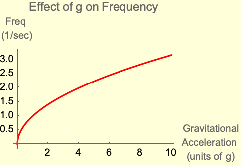
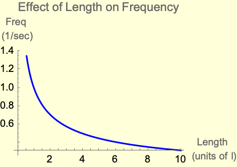
We can plot and algebraically evaluate these relationships for $g$ and $l$ to convince ourselves that our expression makes sense.
- Decreasing $g$ should decrease $f$, since gravity is our only source of acceleration / motion.
- Intuitively, effects of changing $ \ell$ are less clear, so (Eq. 5) proves insightful.
Writing this as an equality rather than a dependency relationship will require us to address any dimensionless constants that would not have been encoded in the dimensionality of $f$. Values like $\pi$ or $1/2$ may appear, and we know that some function of our initial angle $\theta_i$ probably contributes to $f$, since
- an initial angle of zero should give us no pendulum movement: $f(\theta_i = 0) = 0$
- $\theta_i = 90^0$ probably does result in $f_{max}$ since the pendulum sweeps the largest angle (and distance in $\Bbb{R}^3$) at $\theta_i$.
Therefore, we transform (Eq. 4) into an equality by including some unknown function ($\Theta$) of intial-angle: $$ \bbox[8px,border:1px solid black]{f(\ell, g, \theta_i) = \Theta(\theta_i) \sqrt{ \frac{g}{ \ell}}} \tag{Eq. 5}$$
Perfect. We have determined an essential quantity to describe pendulum motion. The contribution to f by our starting angle, $\Theta(\theta)$, can be determined using empirical methods or boundary conditions. In dimensional anylsis, any unitless coefficients or constant will need information from other sources. This should make sense.
Verifying our Work Using Limits of $f(g, \ell)$
To further convince ourselves that (Eq. 5) describes the correct dependencies for $g$ and $\ell$, consider our frequency at extreme inputs; we can use calculus to take interesting limits of $f$ and see if our math "holds up" physically.
$$ \blbox{ \lim_{l \rightarrow \infty} f( \ell) = \Theta \sqrt{g}\ \lim_{l \rightarrow \infty} \sqrt{\frac{1}{l}} = 0 } \tag{Lim. 1}$$Lim. 1 - If $a \lt \lt b$ in a rational ($a/b$), then ($a/b) \rightarrow 0$. Infinite length gives us no motion.
$$ \lim_{l \rightarrow 0} f( \ell) = \Theta \sqrt{g} \ \lim_{l \rightarrow 0} \sqrt{\frac{1}{l}} = \text{Diverges to}\ \infty \tag{Lim. 2}$$
Lim. 2 - $f$ grows as length approaches 0, but $f$ becomes undefined at $l=0$.
This makes physical sense since our pendulum does not exist without length.
Lim. 3 - Zero gravity gives us no pendulum motion. Matches our physical expectation.
Let us finish this off by verifying (Eq. 5) for sure, while determining $\Theta(\theta)$. The Euler-Lagrande equation for motion is best for systems with easily-identifiable energies, as will become clear.
Verify Our Results w/ Euler-Lagrange Equation of Motion